1 Introduction
Modelling the propagation of cosmic ray species through the
interstellar medium is difficult, but worthwhile. A working propagation
model gives a way to predict the spectrum of each species, which lets us
confirm or falsify theories of their origin. It is also a useful place
to look for new production mechanisms, since any persistent disagreement
between model and data points at physics that is not yet in the model.
This post looks at the cosmic ray spectrum of lithium-7 \((^7\text{Li})\), the most abundant isotope of lithium (Tomascak 2004), referred to from here on simply as lithium. Lithium is a secondary cosmic ray species (Vecchi 2021), produced when primary species such as carbon and oxygen spall against the interstellar medium (Yiou et al. 1968). The aim is to fit a model of the lithium spectrum to AMS-02 data by adjusting the diffusion term of the transport equation given below (Strong et al. 2007).
The lithium spectra here come from GALPROP (Strong et al. 2007), a code developed and maintained at Stanford that solves the propagation equation numerically (Strong and Moskalenko 1998). A full description of the solver is out of scope; much of the supporting detail in what follows comes from Strong and Moskalenko, who designed and run GALPROP. Each run varies three free parameters of the spatial diffusion coefficient, which is given by (Strong et al. 2007):
Here \(\beta=\frac{v}{c}\), \(R\) is the rigidity, \(D_{\text{rigid}_\text{br}}\) is the
reference rigidity at which the power law describing the diffusion
coefficient breaks, and \(D_g\) is the diffusion coefficient index,
which takes a different value above and below \(D_{\text{rigid}_\text{br}}\).
Before the high-precision AMS-02 measurements, cosmic ray spectra were generally assumed to follow a single power law. AMS-02 instead showed that every species has a break around \(200\) GV (Venendaal 2020). Using equation 2, the three free parameters \(D_{0_{xx}}\), \(D_g^{(1)}\) and \(D_g^{(2)}\) are fitted to the AMS-02 lithium data. The reference rigidity is held fixed at the GALPROP default, since the break sits at roughly the same rigidity for all the lighter cosmic rays (Yuan et al. 2017).
2 Experimental Results
2.1 Default Values
GALPROP is first run with its default settings: \(D_{0_{xx}}=6.10\times10^{28}\) cm\(^2\) s\(^{-1}\), \(D_g^{(1)}=D_g^{(2)}={1}/{3}\) (the Kolmogorov
turbulence value (Moskalenko 2020)), and \(D_{\text{rigid}_\text{br}}=4.00\) GV.
Figure 2 plots the resulting model alongside the AMS-02 data, comparing
the default settings with and without a solar modulation of \(V=740\) MV. The modulation level is set
using the force-field approximation (Ghelfi et al.
2017), averaged over the AMS-02 operating period via the cosmic
ray database of (Maurin et al. 2020). Figure 1 shows the
resulting time series, from which the average value \(V\approx740\) MV is taken.
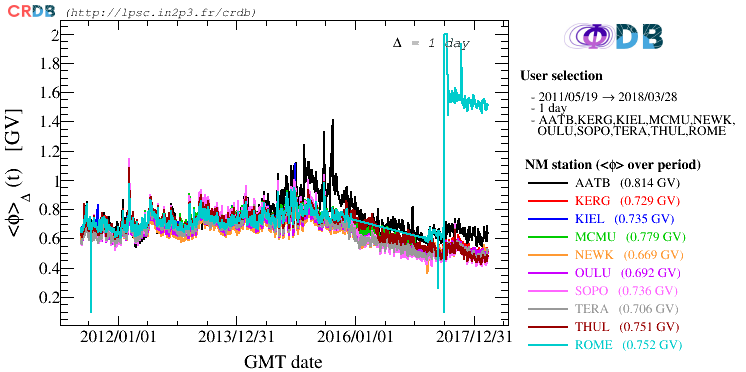
Figure 1 makes it clear that solar modulation varies considerably with time, tracking changes in solar activity. A constant modulation value is used throughout this work; implementing a time-dependent treatment would be a useful extension, but is out of scope here.
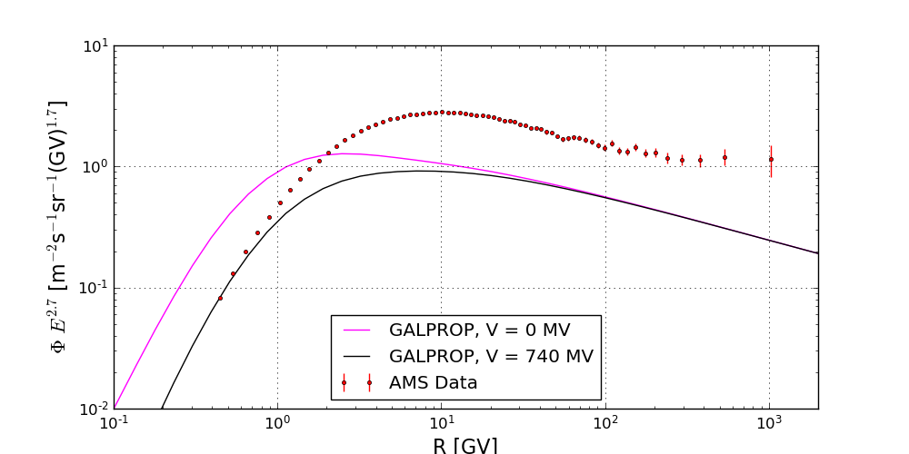
Figure 2 shows that ignoring solar modulation (magenta) produces a
model that does not fit the AMS-02 lithium data at all, while including
it (black) brings the lowest-energy points into agreement. Even with
modulation, however, the default settings fit poorly: GALPROP predicts
a much smaller flux than is observed, and because the diffusion
coefficient index is held fixed at the Kolmogorov value across all
rigidities, the spectrum has no ankle.
Recovering a better fit, and in particular reproducing the ankle, will require non-trivial changes to the three free parameters of the diffusion term.
2.2 Diffusion Term Altered Values
The fit starts from the parameter ranges recommended by Strong and Moskalenko (Strong et al. 2007). They give \(D_{xx}\approx(3-5)\times10^{28}\) cm\(^2\)s\(^{-1}\) at an energy of 1 GeV/n, so \(D_{0_{xx}}\) is fitted within that range. They also give the diffusion coefficient index an empirical range of 0.3 to 0.5, depending on whether the regime is dominated by Kolmogorov (1/3) or Kraichnan (1/2) turbulence (Strong et al. 2007). Because the index depends on the magnetic fields, magnetohydrodynamic waves and discontinuities in the ISM (Strong and Moskalenko 1998), diffusion is in fact highly anisotropic (Strong et al. 2007) and inhomogeneous (Jóhannesson et al. 2016). Splitting the rigidity range into just two regimes is therefore likely too coarse to capture lithium diffusion in detail.
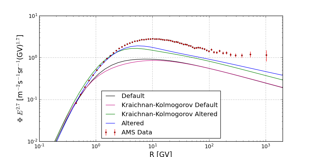
Figure 3 shows the default GALPROP curve (black) alongside a run in
which only the diffusion coefficient indices have been changed, to
\(D_g^{(1)}=1/2\) below the break and \(D_g^{(2)}=1/3\) above it (pink). In other
words, the model now sits in the Kraichnan regime at low rigidity and
the Kolmogorov regime at high rigidity. The green curve uses the same
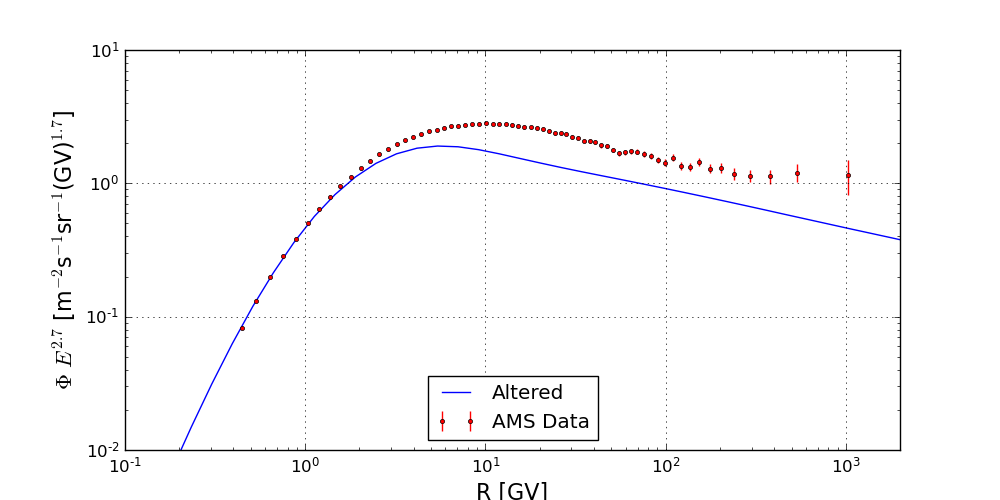
indices but with \(D_{0_{xx}}\) lowered to \(3.75\times10^{28}\) cm\(^2\)s\(^{-1}\). The best fit (blue), shown on its
own in figure 4, was found by varying all three parameters
systematically and lands at \(D_{0_{xx}}=3.75\times10^{28}\)
cm\(^2\)s\(^{-1}\), \(D_g^{(1)}=0.38\) and \(D_g^{(2)}=0.30\). Even this best fit is
poor enough that residual plots are not informative; the discussion
below addresses why fitting GALPROP to lithium through the diffusion
term is so difficult.
3 Discussion
Figure 4 shows the altered GALPROP model still underpredicting the
high-rigidity lithium flux observed by AMS-02. No combination of the
three free parameters tried here was able to recover the high-rigidity
regime. The missing flux is unlikely to come from unaccounted primary
contributions, since GALPROP already includes the relevant channels,
including \(^7\)Be decay via K-capture (Boschini et al.
2020). Lithium produced during Big Bang nucleosynthesis (Hernanz 2015) falls well short of
the cosmic ray amount observed. A more interesting candidate is
explosive lithium production in classical novae, observed for the first
time in V339 Del (Tajitsu et al.
2015); the lithium-rich ejecta from such novae are comparable to
what AMS-02 sees in cosmic rays (Boschini et
al. 2020). Further fits along the diffusion route would
need significantly more constraints, but the persistent shortfall is
itself suggestive of a source that is not yet in the standard
inventory.
The reference rigidity \(D_{\text{rigid}_\text{br}}\) was held
fixed at the GALPROP default rather than treated as a free parameter.
Future fits should let it float, since the AMS-02 break sits at roughly
\(D_{\text{rigid}_\text{br}}\approx 100\) GV (Boschini et al. 2020),
noticeably below the default. Allowing this parameter to vary would
likely improve the overall fit and could also produce a more pronounced
“ankle”, which the altered model here failed to reproduce.
A further difficulty is that lithium behaves quite unlike the other light cosmic ray nuclei. Using carefully fitted parameters for other light species (Jóhannesson et al. 2016) as starting points for the lithium fit gave wildly incorrect results. The fact that lithium is conspicuously absent from the Bayesian analysis of inhomogeneous diffusion in Jóhannesson et al. (2016) is itself a hint that lithium is a problematic species when only diffusion is varied.
4 Conclusion
Fitting the GALPROP model to AMS-02 lithium through the diffusion term alone has been largely unsuccessful, in line with what other authors report; Boschini et al. go as far as calling it the lithium anomaly (Boschini et al. 2020). The contrast with the detailed Bayesian fits achieved for other cosmic ray species suggests that lithium needs more than just diffusion adjustments. Further work should focus on the source term, where there are recent developments in understanding lithium production. Folding those into the source term, alongside the fits to the diffusion term, would have a much better chance of reproducing the AMS-02 data.