1 Introduction
The twentieth century saw the successful development of the Standard Model (SM) of particle physics, one of the most experimentally verified physical theories ever developed (Glashow 1961; Veltman et al. 1972; Weinberg 1972, 1971; Svartholm 1968). The Standard Model predicts the existence of the Higgs boson (Peter Ware Higgs 1964; Peter W. Higgs 1964; Englert and Brout 1964) which for nearly five decades evaded discovery until 2012. The discovery was made as a significant part of the Large Hadron Collider (LHC) research programme and was a significant motivating reason for constructing the world’s largest particle collider (ATLAS Collaboration 2008).
The existence of the Higgs boson is implied by the Brout-Englert-Higgs mechanism. This is the mechanism that spontaneously breaks the gauge symmetry that governs electroweak interactions (Glashow 1961; Englert and Brout 1964; Weinberg 1967). The electroweak symmetry breaking allows other fundamental particles to acquire mass as they interact with the Higgs field (Peter Ware Higgs 1964; Carena and Haber 2003), the Higgs boson is an excitation of this field (Peter Ware Higgs 1964). The first run of the LHC at the centre-of-mass energy \(\sqrt{s}=7\) TeV found the mass, parity, spin and decay modes to be as predicted by the Standard Model (ATLAS and CMS Collaborations 2015; CMS Collaboration 2017, 2018, 2019; ATLAS Collaboration 2019c, 2019b, 2015b, 2022b). LHC runs 2 and 3 are at greater energies, \(\sqrt{s}=13\) TeV and \(13.6\) TeV respectively. New physics within the sensitivity of the data collected at these runs may include particles predicted by the minimal supersymmetric extension of the Standard Model (Lee 1973). The increasingly large statistics generated in these runs could also produce changes and more detailed descriptions of the observables measured in the first LHC run.
Highly precise measurements and analysis systems are required to study any new physics. The first component is the physical detector that measures and records particle collision events at the LHC. The LHC has two general-purpose detectors: the CMS detector (CMS Collaboration, n.d.) and the ATLAS detector (ATLAS Collaboration 2008). This thesis focuses on improving the analysis of \(H\rightarrow\gamma\gamma\) run 2 data captured by the ATLAS detector. Identifying such decays is done by analysing the properties of jets that are clustered using the anti-\(k_T\) algorithm (Cacciari et al. 2008). This field is called jet tagging within high-energy particle physics; different classification algorithms are used to tag the jets. Jet tagging \(H\rightarrow\gamma \gamma\) decays are the focus for several reasons. These decays do not have a jet tagging algorithm of the types developed here. Secondly, the available data is of high quality and quantity, and finally, the interest in increasingly detailed descriptions of the Higgs boson is very high due to its relation to the mechanism by which other particles possess mass. For these reasons, developing \(H\rightarrow\gamma\gamma\) jet tagging algorithms for the ATLAS detector may prove useful tools for physicists at the LHC.
1.1 The ATLAS Detector at the LHC
When the LHC started operations at CERN in 2008, it was the largest particle collider ever constructed (ATLAS Collaboration 2008) and remains so over a decade later. The LHC accelerates groups of up to \(10^{11}\) protons and collides these proton groups together in \(pp\) collisions at a rate of 40 million collisions per second (ATLAS Collaboration 2008). The LHC has been designed to collide protons with a maximum centre-of-mass energy of 14 TeV (ATLAS Collaboration 2008). At such high collision energies, the protons are accelerated to \(99.999999\%\) of the speed of light1. This causes the decay products to become highly collimated (ATLAS Collaboration 2022a). Resolving the strongly boosted decay products requires highly specialised detection hardware and software.
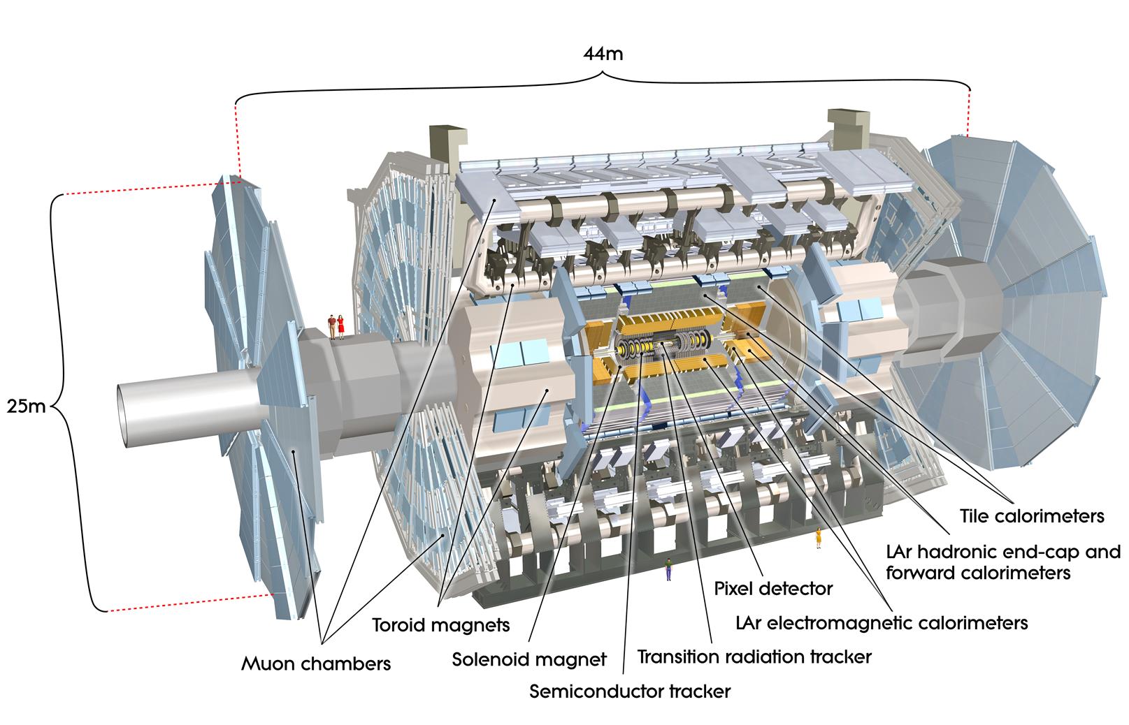
The state-of-the-art hardware that forms the centre of this work is the ATLAS (A Toroidal LHS ApparatuS) detector2 (ATLAS Collaboration 2008), the device that generates data from collisions that will be the focus of this paper. The multipurpose ATLAS detector nearly surrounds the collision point in cavern 1 of the LHC (ATLAS Collaboration 2008, 2022c). It comprises several critical components designed for high-precision measurements, as seen in the cut-away model in Figure Fig. 1. First, an inner tracking detector is surrounded by a solenoid that provides a powerful axial magnetic field that enables the tracking of charged particles in conjunction with silicon-pixel detectors (ATLAS Collaboration 2012) and the transition radiation tracker (TRT) (ATLAS Collaboration 2008). The TRT is vital as it provides electron identification information (ATLAS Collaboration 2022c). The next major system within the ATLAS detector is the calorimeter system, which consists of electromagnetic and hadron calorimeters. Electromagnetic calorimetry is achieved with high-granularity lead/liquid-argon (LAr) and copper/LAr calorimeter modules depending on location within the ATLAS detector (ATLAS Collaboration 2008). Hadron calorimetry uses steel/scintillator-tile calorimeters and tungsten/LAr calorimeters (ATLAS Collaboration 2008, 2022c). Finally, a muon spectrometer relies upon three superconducting air-core toroidal magnets that provide vast magnetic fields to deflect negatively charged muons for high-precision tracking.
When in operation, the ATLAS detector records collision events at a rate of 200 Hz (ATLAS Collaboration 2008) and records many different variables for each event. These data must then be analysed and the collision events categorised. This stage requires dedicated jet tagging algorithms for the particle decay being studied.
1.2 Photon Identification
Naturally, the ATLAS detector component that is primarily involved in photon reconstruction and identification is the electromagnetic calorimeter (ATLAS Collaboration 2008). As photons interact with the material of the calorimeter, an electromagnetic shower is created and deposits its energy in a small group of neighbouring calorimeter cells (ATLAS Collaboration 2016). The signatures of photons and electrons are similar, so reconstruction for both these particles occurs in parallel. Due to the similarity between photons and electrons, discriminating between the diphoton signal class and the electron background classes is important to any jet tagging algorithm focussing on a photon decay product signal.
The standard ATLAS reconstruction of photons is done by first searching for seed clusters in the calorimeter cells (ATLAS Collaboration 2016). How these clusters are created has been a significant source of research and development, resulting in the widely used superclusters (ATLAS Collaboration 2019a). These are dynamic and variably sized seed clusters and have improved the ability to recover energy carried by photons generated by bremsstrahlung, or electron or photon conversions (ATLAS Collaboration 2019a). There are two types of detectable photons: the converted and the unconverted. Converted photons are those that interact with a charged particle, such as an atomic nucleus, and convert into an electron-positron pair (Bishara et al. 2014). Unconverted photons are those that do not undergo this process. Converted photons can be tracked, and their superclusters are matched to a conversion vertex (or vertices) (ATLAS Collaboration 2019a). Unconverted photons are superclusters that are not matched to a conversion vertex nor any track information (ATLAS Collaboration 2016, 2019a).
From this information, the ATLAS standard method for photon identification uses one-dimensional selection criteria that are based on electromagnetic shower shape feature variables (ATLAS Collaboration 2019a). This cut-based selection approach is designed to select photons efficiently and reject backgrounds (ATLAS Collaboration 2019a). Primary identification is done at a Tight operating point, with less restrictive operating points (Medium and Loose) used as triggers for the ATLAS detector (ATLAS Collaboration 2019a). Tight photon identification is performed separately for converted and unconverted photons as their associated showers are topologically distinct. This is a result of the conversion electron-positron pair, which are electrically charged, resulting in deflection caused by the powerful magnetic field within the ATLAS detector (ATLAS Collaboration 2019a).
The ATLAS standard method for photon identification performs well over a large kinematic range; however, for highly boosted \(H\rightarrow\gamma\gamma\) decays, the performance significantly degrades. This is due to the aforementioned Lorentz boosting of heavy boson decay products (Sharp 2016), causing the angular distance between decay products to be reduced. The angular distance of two decay products is inversely proportional to the transverse momentum3 (ATLAS Collaboration 2022a). Therefore, greater momentum due to larger velocities leads to smaller angular distances.
To develop identification algorithms at the top end of the kinematic range is extremely important, especially as Run 3 is underway at the LHC at the higher centre-of-mass energy of \(\sqrt{s}=13.6\) TeV (S. Fartoukh et al. 2021). Therefore, a larger proportion of highly boosted heavy bosons will be produced for detection in the ATLAS detector in the near term. A class of identification algorithms using deep neural networks has recently been effective for other highly boosted heavy bosons.
1.3 Deep Neural Networks
Deep neural networks (DNNs) are a broad class of algorithms capable of classification and regression depending on the architecture and downstream task. DNNs are characterised by possessing input and output layers with several so-called hidden layers between them (Nielsen 2015). The hidden layers consist of hidden nodes, performing linear and non-linear transformations on the input data and mapping it to the output (Nielsen 2015). An optimisation algorithm, which since the 1980s has been some form of stochastic gradient descent (Rumelhart et al. 1986), iteratively adjusts the weights and biases of the hidden nodes (Nielsen 2015). This is done during the backpropagation step to minimise an objective (loss) function that is carefully chosen for the task (Rumelhart et al. 1986; Nielsen 2015). These networks automatically and adaptively learn hierarchies in the feature variables, enabling the network to capture complex representations of the input data (Nielsen 2015).
DNN jet tagging algorithms have recently been utilised for particle identification using the ATLAS detector. Successfully developed DNN algorithms include those for identification and reconstruction of hadronic boson decays (CMS Collaboration 2020), decays into boosted di-\(\tau\) systems (ATLAS Collaboration 2020) and for highly boosted \(Z\rightarrow e^+ e^-\) decays (ATLAS Collaboration 2022a).
As mentioned in Section 1.2, electron and photon identification are closely related due to the similarity in their signatures in the electromagnetic calorimeter (ATLAS Collaboration 2016). Therefore, the approach to identifying \(Z\rightarrow e^+e^-\) decays is extremely relevant for this thesis. Similar techniques are used to identify both of these highly boosted decays.
1.3.1 Mass Decorrelation with Adversarial Neural Networks
The power of DNNs when presented with complex input data is that they are highly able and flexible when learning how to map the inputs to outputs. However, in the case of jet tagging, highly useful topological jet features are strongly correlated to the jet mass (Dolen et al. 2016). This can result in the DNN over-relying on the mass feature, underutilising the jet substructure information and increasing systematic uncertainty as signal efficiency degrades at less frequent signal masses (C. Shimmin et al. 2017). It leads to sculpting of the backgrounds dependent on the signal mass distribution. As the relationship between the mass feature and other topological features is complex and extremely difficult to characterise.
One successful approach has been to add a second DNN to act as an adversary to train the jet tagger to be invariant to the mass (C. Shimmin et al. 2017). The jet tagger learns to classify the jets in the input data; the adversary network then takes the output from the jet tagger and attempts to predict the binned mass value (C. Shimmin et al. 2017). The adversary is optimised on its ability to make this mass prediction, whilst the jet tagger is optimised on the combination of its classification loss function and the adversary loss (C. Shimmin et al. 2017). This training scenario is termed an adversarial neural network (ANN).
Incorporating mass decorrelation into the training strategy of a jet tagger is an effective method for reducing the sensitivity to the systematic uncertainties derived from the dominance of the mass feature (C. Shimmin et al. 2017). Whilst achieving the primary goal of high jet tagging performance (C. Shimmin et al. 2017).
1.4 Research Objectives
Given the complexity of the task and its importance to high-energy particle physics research, looking beyond the Standard Model, this thesis undertakes two primary objectives to advance the jet tagging of \(H\rightarrow\gamma\gamma\) decays.
Improve highly boosted \(H\rightarrow\gamma\gamma\) decay identifications using deep neural networks.
Develop a deep neural network that makes its \(H\rightarrow\gamma\gamma\) identifications decorrelated from the mass feature of the input data. While maintaining a high degree of discriminatory power.
Achieving these objectives could substantially contribute to both theoretical and experimental particle physics by enhancing jet tagging capabilities and minimising biases.
The paper is organised as follows: Chapter 2 elaborates on the methodology, providing information on the simulated dataset, exploratory data analysis, feature analysis, network architectures, and evaluation methods. In Chapter 3, detailed results of the models’ performance are reported. Chapter 4 discusses these results and possible routes for future research. Finally, Chapter 5 offers conclusive remarks on this thesis’ results, implications and potential contributions to the field.
2 Methodology
This chapter presents the methodology for developing and evaluating the jet tagging algorithms. Initially, the data utilised for the study is discussed, beginning with its acquisition. Justification for the before-experimentation selection of features within the dataset is also provided. After this, an examination of exploratory data analysis is conducted, scrutinising the attributes of the data with respect to the target classes. Feature analysis follows, elaborating on the significance of various features in influencing the performance of the final models. The mass feature is examined in detail due to one of the stated aims of developing a mass-decorrelated jet tagger. Finally, the architectures of the neural networks are presented along with their underlying rationale, and the evaluation methods applied to assess the jet tagging algorithms are detailed.
2.1 Data
Acquiring high-quantity and quality data is fundamental in developing classification algorithms employing machine learning techniques like deep neural networks. When trained on robust datasets, such neural networks exhibit high flexibility and expressiveness, enabling them to capture complex and nonlinear relationships between input features and output targets (Basu et al. 2010). For the purposes of this study, data generated through Monte Carlo event simulation is utilised. This is a methodology commonly employed in the domain of high-energy particle physics (Gleisberg et al. 2004; Gleisberg et al. 2009; E. Bothmann et al. 2019; J. Alwall et al. 2007; J. Bellm et al. 2016; T. Sjöstrand et al. 2015).
2.1.1 Monte Carlo Event Generation
Monte Carlo event generation is a broad computational technique employed to simulate complex systems and processes by generating random samples from known distributions (James 1980). Instead of attempting deterministic calculations following classical equations, probability distributions are defined, and samples from these distributions are randomly sampled. This method can be applied to deterministic but highly complex scenarios where analytic solutions are intractable. Naturally, it can also be applied to the simulation of quantum particles and their interactions, an inherently stochastic process (James 1980).
In this thesis, simulated data from three MC event generators,
SHERPA (E.
Bothmann et al. 2019), MadGraph (J. Alwall et al. 2007),
and PYTHIA8.3 (C. Bierlich et al. 2022) are employed for
the training of jet tagging algorithms. The feature variables in the
simulated data are those measurable and capable of being recorded by the
ATLAS detector at the LHC (ATLAS Collaboration 2008). Information
for the generation of specific particle collision events, namely the
signal \(H\rightarrow\gamma\gamma\)
decays and background noise \(Z\rightarrow
e^+e^-\) decays, \(q/g\)-jets,
\(e/\gamma\)-jets, and \((\tau)\tau\)-jets, are included. These
datasets are thus utilised to develop jet tagging algorithms compatible
with actual data from the ATLAS detector.
It should be noted that the simulated dataset is divided into three segments. Comprising 60% of the total number of events is the training dataset, while validation and testing segments each constitute 20% of the data. In the training dataset there are around 280,000 \(H\rightarrow\gamma\gamma\) decays, 2.3 million \(Z\rightarrow e^+e^-\) decays, 3.7 million \(q/g\)-jets, 1.6 million \(e/\gamma\)-jets and 700,000 \((\tau)\tau\)-jets. All analytical procedures and model training are conducted on the training dataset. Performance checks during the training phase are carried out using the validation dataset. Lastly, the testing dataset is reserved exclusively for the final evaluation of the models.
2.1.2 Features
Previous work on other decay processes uses the tracking information provided by the ATLAS detector’s inner tracking detector (ATLAS Collaboration 2008, 2022a). As photons have zero electric charge, they undergo no deflection due to the solenoid’s magnetic field (ATLAS Collaboration 2008), calorimeter information is more relevant. Due to the reduced utility in the tracking features for the signal process \(H\rightarrow\gamma\gamma\), the training data contains significantly fewer features than previous work on different decay processes (ATLAS Collaboration 2022a). The feature variables that data has been MC generated for are provided in Table 1.
| Feature | Description |
|---|---|
| \(p_T\) Bin | Binned transverse momentum of the jet. This momentum component is perpendicular to the direction of the particle beam in the collider. |
| \(|\eta|\) Bin | Binned absolute pseudorapidity of the jet. Pseudorapidity is a spatial coordinate that describes the angle of a particle relative to the beam. \(\eta=-\ln{\tan{(\theta/2)}}\) where \(\theta\) is the polar angle with respect to the anticlockwise beam direction (V. Khachatryan et al. 2010). |
| \(m\) | Mass of the jet. |
| \(\Delta R (c_1,j)\) | Angular distance of the leading cluster to the jet axis. |
| \(\Delta R (c_2,j)\) | Angular distance of the sub-leading cluster to the jet axis. |
| \(\Delta R (c_1,c_2)\) | Angular separation between the two leading clusters. |
| \(r^{(\beta=1)}_{N=1}\) | Ratio of the energy correlation functions calculated from the two leading tracks (ATLAS Collaboration 2022a; Larkoski et al. 2013). This is sensitive to the jet’s \(N\)-prong substructure (Larkoski et al. 2013). |
| \(\max{\big(\frac{E_{{layer}}}{E_{{jet}}}\big)}\) | Maximum fraction of energy deposited by a jet in a single layer of the EM calorimeter (ATLAS Collaboration 2015a). |
| \(f_{{EM}}\) | Fraction of energy deposited in the EM calorimeter (ATLAS Collaboration 2015a). |
| \(E/p\) | Ratio of the cluster energy to the track momentum (ATLAS Collaboration 2022a). |
| Planar Flow | Spread of the jet’s energy over the area of the jet calculated from the two leading tracks. Values around 1 indicate an even spread, and values around 0 indicate a linear spread (ATLAS Collaboration 2022a). |
| Width | Width of the jet, defined as the \(p_T\) weighted average of the \(\Delta R\) distances between the neutral particle flow objects and jet axis direction (ATLAS Collaboration 2022a). |
| Balance | The ratio of the difference between cluster energies and the total energy of the clusters \(\frac{E^{{1st}}_{{cluster}}-E^{{2nd}}_{{cluster}}}{E^{{1st}}_{{cluster}}+E^{{2nd}}_{{cluster}}}\). |
| \(N^{Const.}\) | Multiplicity of particle-flow objects per jet. |
| \(N^{{Trk}}\) | Multiplicity of tracks per jet. |
2.2 Exploratory Data Analysis
In this section, the features are initially visualised in a couple of ways to investigate the inherent distribution of the data in the features with respect to the target classes.
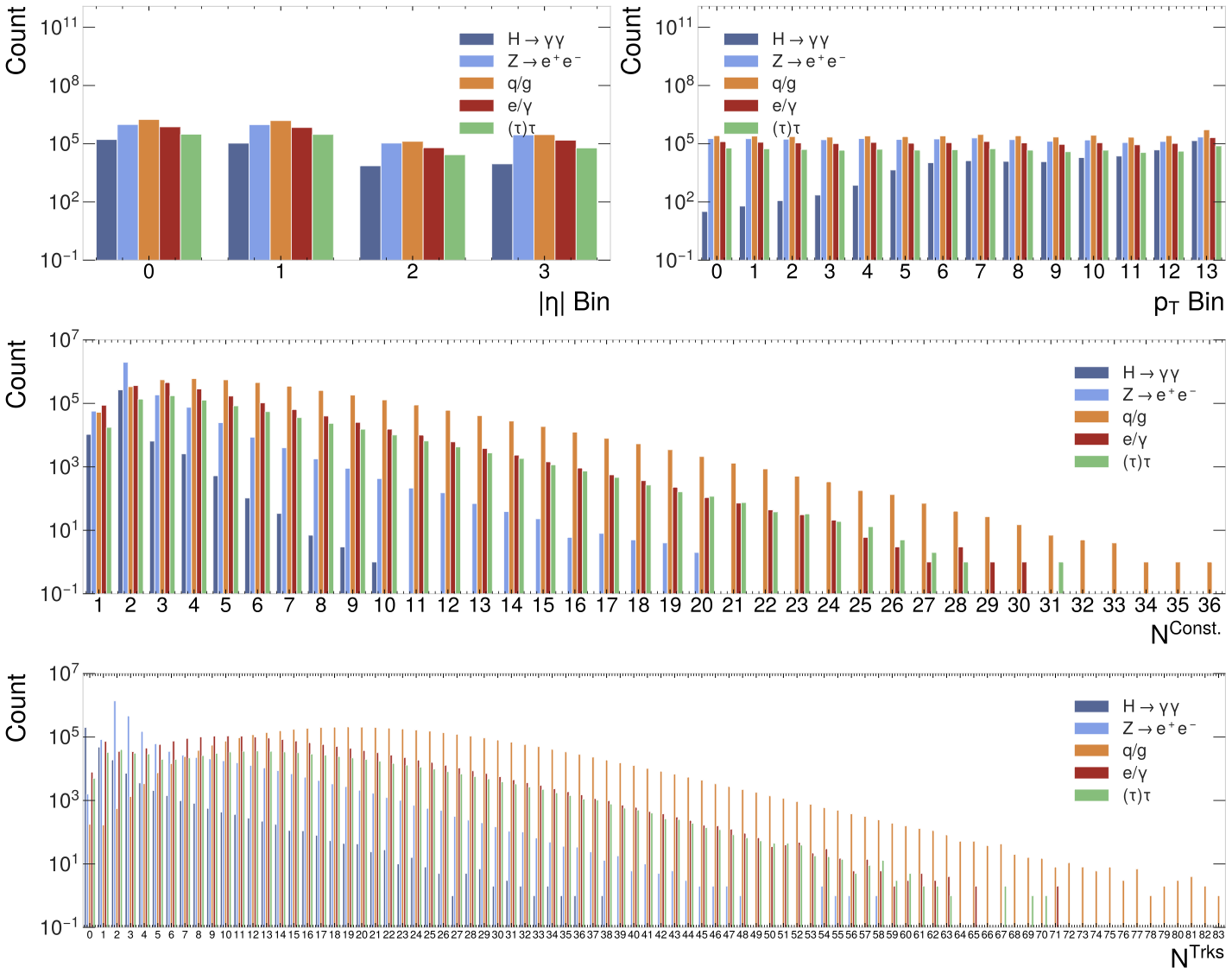
As there are continuous and categorical feature variables, the analyses are separated to present the most relevant plots and information to the feature type. Figure Fig. 2 contains four bar plots, one for each categorical variable. Each bar plot within the figure illustrates the frequency distribution of each feature across the different types of particle collision events. In absolute terms, the signal process is less frequent than the background processes.
First, consider the top row plots in Figure Fig. 2; these show the frequency distributions across decay types of \(|\eta|\) bin and \(p_T\) bin features. In the \(|\eta|\) bin plot, all classes are most numerous in the first two bins, but overall, the distribution is quite flat. The \(p_T\) bin bar plot shows that the distribution of all the background jets is relatively flat, but the distribution of the signal jets increases as the bin index increases. Pseudorapidity and transverse momentum are highly dependent on the energy of the particle beam in the LHC. The classifiers should be able to function within a range of beam energies. This will require the decisions of the classifier models to be decorrelated with respect to these features. How this will be implemented will be described in section 2.4 when the network architectures are presented.
Two similar distributions can be observed in the bar plots for the \(N^{Trks}\) and \(N^{Const.}\). The signal jets are only significant in relatively low bin indices compared to the total number of bins. The background jets all have significantly greater spreads across the bins. This suggests that these will be useful features to the jet taggers for distinguishing the signal from the background jets.
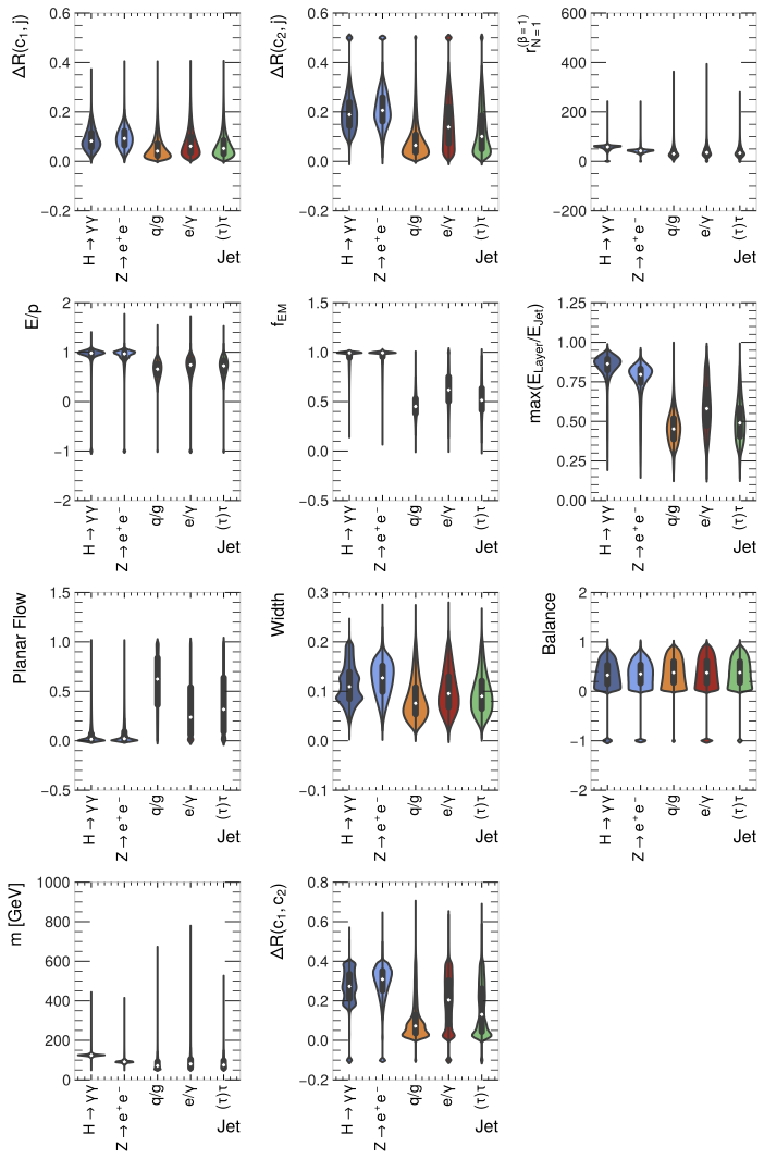
The ten continuous feature variables are visualised against the target classes using violin plots in Figure Fig. 3. These plots allow the distribution and the probability density of the data for each feature to be displayed simultaneously. It should be noted that the most significant outliers in all plots comprise the default values for the feature variable; these are recorded when a measurement for this feature cannot be made. The default values for individual feature variables that possess them are contained in Appendix Eq. 1..
The violin plots for the signal jets are similar to the \(Z\rightarrow e^+e^-\) background decays. Across all features, the signal process and \(Z\rightarrow e^+e^-\) decays have the most qualitatively similar distributions and probability densities. It should be noted, however, that the signal process has some slightly more complex probability densities for the width and the \(\Delta R (c_1,c_2)\) features. The implication is that the classifiers will find discriminating the signal jet from the Z-boson background jet the most difficult.
Additionally, the other background jets possess even more similar violin plots to one another across all features. The jet taggers, therefore, may find discriminating background jets from one another an even harder task. This is not a significant issue, as correctly identifying the signal jet and reducing background jets is the main aim of this thesis.
From Figure Fig. 3, the continuous feature variables that will likely be of greatest utility to the deep neural networks as they are learning to discriminate between the different decay processes are \(r^{(\beta=1)}_{N=1}\), \(E/p\), \(f_{EM}\), \(\max{(E_{layer}/E_{jet})}\) and mass. This is due to the median, interquartile range and probability density of the signal class in these features being the most different from the background classes. The second jet tagger aims to identify the signal jet decorrelated to the mass feature. As the mass feature clearly contains highly useful information to the network, developing a mass-decorrelated network requires specific architecture decisions; these will be further discussed in section 2.4. However, seeing the information in the mass violin plot indicates this task’s difficulty.
Finally, for the continuous features, it is noted that the features shown with the least utility displayed within the violin plots are the features where the distributions and probability densities are most similar across all jets. This is seen most evidently in the violin plot for the balance; to a lesser degree, it is also observed for the planar flow. These features likely contain limited useful information for the classifiers.
2.3 Feature Analysis
This section analyses the features via correlation coefficients and the mutual information metric. Furthermore, the relationship between various feature variables and the mass feature is examined in more detail, given the objective of decorrelating the second model’s classification from this particular feature.
2.3.1 Correlation Coefficients
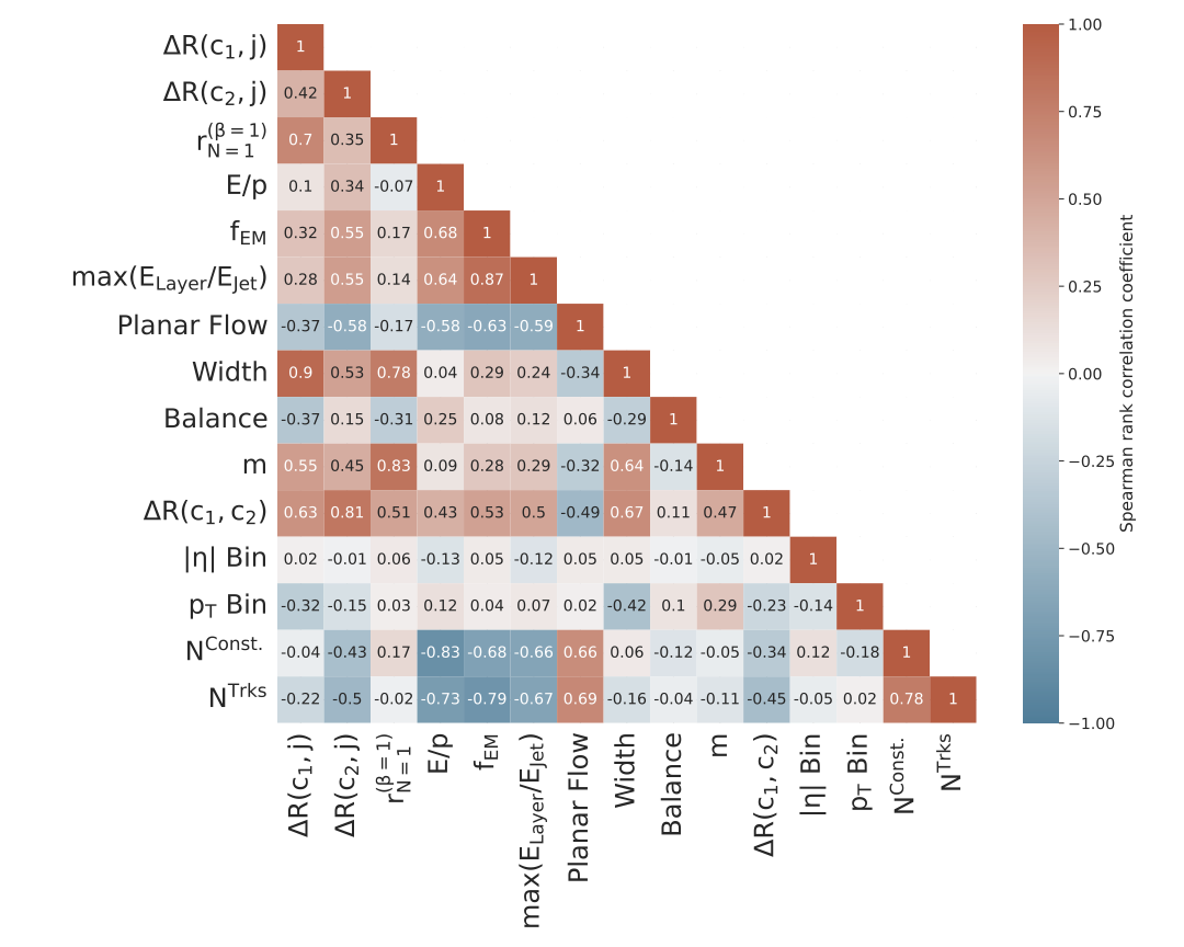
A succinct method for examining correlations between features is to use a correlation coefficient matrix as seen in Figure Fig. 4. This figure displays a matrix of the features and their corresponding Spearman rank correlation coefficient. This nonparametric measure enables the calculation of correlation for general monotonic relationships and is deemed suitable for scenarios where nonlinear correlations are anticipated (Tsanas et al. 2012). The range of this correlation coefficient is [-1,1]; positive values are interpreted as positively correlated, and negative values as negatively correlated, 0 indicates no correlation (Tsanas et al. 2012).
Notably, the binned absolute pseudorapidity (\(|\eta|\) bin) and the binned transverse momentum (\(p_T\) bin) of the jet have relatively small correlation coefficients with all other features, especially \(|\eta|\) bin. This suggests that these features contain significant information not present in the other features. As expected, the mass is the largest positive correlation for the \(p_T\) bin feature.
More generally, many features correlate positively or negatively to many other features in the data. The relationship between the features and the target classes is complex and motivates the use of a type of classifier that is highly expressive.
2.3.1.1 Mass Feature Correlations
Decorrelating the identification made by a classifying model from the mass feature variable can be attempted in several ways. However, the decision of which method to use is related to how many relationships this feature has with other features. The more correlated the mass feature is to other features, the more complex the relationship, requiring more complicated network architecture and training decisions.
As seen in Figure Fig. 4, the mass feature (\(m\)) has a Spearman rank correlation coefficient with an absolute value greater than 0.25 with 9 of the other features. It has a value greater than 0.5 for 3 of the features. As expected, the features that mass is most strongly correlated to are topological features of the jet \(\Delta R (c_1,j)\), \(\Delta R (c_2,j)\), \(\Delta R (c_1,c_2)\), \(r^{(\beta=1)}_{N=1}\) and width. Making jet identifications from the associated but distinct jet topology will allow the mass-decorrelated classifier to perform at a greater range of energies.
The relationship of the mass with other features is clearly complex and, therefore, requires a high-capacity network architecture to achieve mass invariance and a high level of signal accuracy. This contrasts the binned pseudorapidity and transverse momentum features, which are not strongly correlated to many, if any, in the case of pseudorapidity.
2.3.2 Mutual Information
In the previous section, the correlation between features was determined; in this section, another metric to rank the features by a single score is employed. Such a method for measuring the relative importance of different features is mutual information. This metric determines relevance and redundancy between features and the target class (Estévez et al. 2009). Mutual information is a nonparametric measure that is useful in nonlinear settings (Kraskov et al. 2004), such as this complex ATLAS detector data scenario. The metric has a range \([0,\infty)\) and is only 0 if and only if the two random variables in question are independent (Kraskov et al. 2004). The equations for both random discrete and continuous variables are presented in equations Eq. 3. and Eq. 4. respectively (Kraskov et al. 2004). Where \(p(x,y)\) is the joint probability density function (pdf) and, \(p(x)\) and \(p(y)\) are the marginal pdfs of random variables \(X\) and \(Y\).
| Feature | MI Score | Feature | MI Score |
|---|---|---|---|
| \(N^{Trks}\) | 0.63 | \(\Delta R(c_2,j)\) | 0.24 |
| \(f_{EM}\) | 0.54 | \(r^{(\beta=1)}_{N=1}\) | 0.21 |
| \(\max{\frac{E_{layer}}{E_{jet}}}\) | 0.43 | \(|\eta|\) Bin | 0.12 |
| \(N^{Const.}\) | 0.39 | \(\Delta R(c_1,j)\) | 0.11 |
| \(E/p\) | 0.34 | Width | 0.10 |
| \(m\) | 0.34 | \(p_T\) Bin | 0.06 |
| Planar Flow | 0.30 | Balance | 0.02 |
| \(\Delta R(c_1,c_2)\) | 0.29 |
Overall, the MI values in Table 2 are somewhat low. This suggests that the features are not highly predictive in isolation. Figure Fig. 4 certainly suggests that the features possess many relations to one another, suggesting that there are likely complex relationships amongst the features and then with the target variable. Another possible interpretation is there is an inherent complexity to the target variable. The target variable is the decay process caused by strongly boosted particles in the LHC; this is subject to a range of physical processes, meaning the target variable is inherently complex.
If there were significantly more features, the MI score could be used as a feature selection method to remove the least relevant features. As previously stated, no features will be pruned due to the relatively low number. This, combined with the analysis suggesting that there are complex relationships between feature variables and the target variable, means that it is prudent not to prune these features from the set of input variables for the neural networks.
The next section will outline the network architectures and the training procedure under which the classifiers will learn to tag the highly boosted \(H\rightarrow\gamma\gamma\) decays.
2.4 Network Architectures and Training Procedure
This thesis aims to produce a dedicated jet-tagging algorithm for the strongly boosted \(H\rightarrow\gamma\gamma\) decay process as measured and recorded in the ATLAS detector in the LHC. In section 2.4.1, the methodology for developing this algorithm is provided, along with its architecture and training procedure. Section 2.4.2 contains the same information for developing a mass-decorrelated jet-tagging algorithm and highlighting the key differences between the two classifiers.
It should be noted that the \(q/g\)-jets have also been removed from the data for both classifiers. This provides the jet-tagging algorithms with a classification task between four jets as performed in previous related work (ATLAS Collaboration 2022a). This will make comparison to previous work more relevant and meaningful. These jets are selected for removal due to their relative lack of importance for confusion with the signal jet and the fact that it is the most numerous class; removing \(q/g\)-jets aids in addressing the class imbalance. Five-class jet taggers are developed and presented in Appendix Eq. 5..
All networks are constructed using the PyTORCH (A. Paszke et al. 2019)
package and are defined using the associated framework. All training
uses an Nvidia A100 GPU with 20Gb of memory and 32 CPU cores (Edinburgh 2023).
2.4.1 DNN
The architecture for this network is based on a recent work dedicated to another heavy boson decay at the same collision energy in the LHC using the ATLAS detector. This jet-tagging algorithm was developed for \(Z\rightarrow e^+e^-\) decays (ATLAS Collaboration 2022a). This decay has been identified in the exploratory data analysis as the background class most likely to be confused for the signal jet \(H\rightarrow\gamma\gamma\). Therefore, the classifying algorithm for the boosted Z-boson decay is a good architecture to base the H-boson decay classifier, as it has been proven to perform well for a similar decay process. This architecture is a fully-connected feedforward deep neural network (ATLAS Collaboration 2022a; Sanger 1989).
The network uses all features as input variables; thus, it has 15 input variables. These data pass through the hidden layers that are composed of nodes with four outputs corresponding to the four target classes, the signal \(H\rightarrow\gamma\gamma\) decays and the three backgrounds, \(Z\rightarrow e^+e^-\) decays, \(e/\gamma\) and \((\tau)\tau\)-jets. These output nodes are the calculated probabilities for the jet in question to be attributed to one of the classes. Each hidden layer has an activation function; the two functions that are tested are the Sigmoid activation function (D.E. Rumelhart et al. 1985) and the rectified linear unit (ReLU) (Nair and Hinton 2010). The sigmoid activation function is the best-performing function in one of the previous works (ATLAS Collaboration 2022a) and ReLU in another relevant work (C. Shimmin et al. 2017). Thus, these activation functions will be trialled for the DNN jet tagger. The weights in the network are initialised with the widely used Glorot initialisation technique (Glorot and Bengio 2010). This initialisation method draws the initial weights from a zero-mean Gaussian distribution (Glorot and Bengio 2010). It has particular utility when used with symmetric activation functions around zero, such as the sigmoid activation function applied to each layer. Batch normalisation is also applied to each hidden layer (Ioffe and Szegedy 2015). This normalises layer inputs, reducing internal covariate shift. This makes the networks less sensitive to the specificities of random weight initialisation and accelerates the learning rate as convergence becomes easier (Ioffe and Szegedy 2015).
For training the multiclass classification loss function,
cross-entropy loss is used (Goodfellow et al. 2016). This
function is weighted by the proportions of each jet to address the class
imbalance within these data. The loss function is additionally weighted
so that the \(p_T\) and \(|\eta|\) bins have a flat distribution. The
method for stochastic optimisation used is the popular ADAM
optimizer (Kingma and
Ba 2017).
To mitigate the risk of overfitting, the dropout method for regularisation is applied to the hidden nodes (Srivastava et al. 2014). During training, a fraction of the nodes are randomly switched off so that the network becomes less sensitive to the specific weight of the nodes (Srivastava et al. 2014). At inference time, the output of each node is scaled down by the dropout rate to account for the missing activations during training (Srivastava et al. 2014). Additionally, early stopping is employed to reduce overfitting (Prechelt 2002); training is stopped after five epochs with the loss decreasing by less than \(10^{-4}\).
To find a set of optimal hyperparameters, ranges are defined for each hyperparameter, and then a grid search is performed over all combinations of the hyperparameters (Bergstra and Bengio 2012). The optimisation range for each hyperparameter is seen in Table 3, where possible, the computational expense is reduced by narrowing ranges by utilising found values in the related work (ATLAS Collaboration 2022a). The top five models are found based on their cross-entropy loss on the validation dataset and are compared to one another using the evaluation methods presented in section 2.5 to find the best-performing DNN jet tagger.
| Hyperparameter | Optimisation Range |
|---|---|
| Training epochs | [30, 50] |
| Optimiser | Adam |
| Dropout probability | [0.01, 0.1] |
| Learning rate | [0.001, 0.01] |
| Hidden layers | [3,4] |
| Hidden nodes | [100, 200] |
| Activation function | [Sigmoid, ReLU] |
2.4.2 Mass-Decorrelated Adversarial Network
The second jet-tagging algorithm is developed in much the same way as the DNN classifier. The fundamental difference comes from having a classifying network and an adversary network. The classifying network architecture is essentially the same as the DNN classifier; the classifier is presented with the input feature data and then attempts to predict the class the jet belongs to. The softmax activation function (Gao and Pavel 2017) is then applied to the outputs; these outputs are passed through the adversary network, which attempts to predict the mass. The loss function is then a linear combination of the loss functions for both the classifier and adversary networks (C. Shimmin et al. 2017), as seen in equation Eq. 6.. The coefficient \(\lambda\) is a positive constant and is a hyperparameter that must be determined in the hyperparameter optimisation. The \(\lambda\) value found in the previous work is \(\lambda=100\) (C. Shimmin et al. 2017); this conveniently narrows the range required for hyperparameter optimisation. This type of neural network is termed an adversarial neural network (ANN) training setup.
The complex relationships explored in the feature analysis in section 2.3 motivate using a flexible neural network that can learn these relationships implicitly between the class and mass and mass-related features. This contrasts the transverse momentum and pseudorapidity features that do not correlate with other features to anywhere near the same degree. Producing jet taggers decorrelated to these features can be managed by weighting the loss function to have a flat distribution with respect to both these features.
The network architecture and training implemented extends previous work for mass-decorrelated jet taggers (C. Shimmin et al. 2017). Following this approach, both networks use the cross-entropy loss function (C. Shimmin et al. 2017). The mass feature is transformed from a continuous feature variable to a categorical one. Ten mass bins are created, each with an equal number of samples. The classifier loss function is again weighted to have flat distributions with respect to the transverse momentum and pseudorapidity bins. The adversary loss is weighted so that signal jets have weight zero, thus becoming invisible to the adversary network (C. Shimmin et al. 2017). This leads to a more challenging situation for the classifier network as it attempts to outperform the adversary without directly relying on the mass feature.
Nearly all hyperparameters are identical to the ones used in the DNN classifier, except there are now two networks with hyperparameters to determine. However, there is an additional hyperparameter, the aforementioned \(\lambda\). It should also be noted that the adversary network is less complex than the classifier, as in the related work (C. Shimmin et al. 2017). This allows the classifier to outperform the adversary as the training progresses so that the classifier is what is developed and not a highly competent mass predictor (C. Shimmin et al. 2017). The hyperparameter space is seen in Table 4.
The adversary is also pre-trained (C. Shimmin et al. 2017) for five epochs to learn an initial representation of the data distribution from the training dataset. Additionally, to ensure that all mass bins contain sufficient signal jets for the adversarial setup to function across mass values, the training dataset is oversampled (Japkowicz and Stephen 2002). This functionally increases the size of the training dataset and, therefore, the computational cost. This occurs in tandem with the added cost of an additional network to optimise; the resulting impact is that the resource constraint reduces the number of hyperparameter combinations that can be searched over compared to the DNN architecture.
The top five model hyperparameter configurations are found by calculating the mean and standard deviation of the signal efficiency across the mass bins. A maximum threshold for the validation loss is set at 0.4, and a maximum threshold for the standard deviation of the signal efficiency is set to 0.2. The top five models then satisfy these threshold criteria and have the highest mean signal efficiency across the mass bins.
In the next section, the criteria by which the DNN and adversarial jet taggers are evaluated are presented.
| Hyperparameter | Optimisation Range |
|---|---|
| \(\lambda\) | [0.01, 100] |
| Training epochs | [30, 50] |
| Optimiser | Adam |
| Dropout probability (C) | 0.01 |
| Learning rate (C) | [0.001, 0.01] |
| Hidden layers (C) | 4 |
| Hidden nodes (C) | 200 |
| Activation function (C) | [Sigmoid, ReLU] |
| Learning rate (A) | [0.01, 1] |
| Hidden layers (A) | 4 |
| Hidden nodes (A) | [100, 200] |
| Activation function (A) | [Sigmoid, ReLU] |
2.5 Evaluation methods
Various evaluation methods are employed to determine the performance of the jet taggers in both a qualitative and quantitative manner. As mentioned in section 2.4, the cross-entropy loss is calculated on the validation dataset so as to have an online evaluation of the networks during hyperparameter optimisation. The aim is to minimise this loss; the five models in each hyperparameter optimisation with the smallest validation loss values are compared using this section’s remaining criteria. The offline evaluation criteria use the held-out test dataset, which is the same size as the validation dataset.
The first evaluation metric is the confusion matrix. This enables a comparison between the model’s performance and the actual data values, clearly visualising which classes the model tends to misclassify and what those mistaken classes are. Ideally, the jet taggers are confident and correct in all classes. However, it is signal class accuracy that is primarily desired. In the event of background class confusion, this is not an issue. Additionally, the confusion matrix will provide information about misclassifications, aiding interpretation as to the cause of confusion.
The area-under-curve (AUC) value for the receiver-operating characteristics (ROC) curves will also be calculated and tabulated. The ROC curve represents the true positive rate (TPR) against the false positive rate (FPR) for different classification thresholds. The AUC metric computes the area under the ROC curve. It provides a scalar value that quantifies the overall ability of the model to discriminate between the positive and negative classes. A perfect classifier will have an AUC of 1, while a random classifier will have an AUC of 0.5. These are useful metrics to assess the jet taggers holistically.
The next metric allows the assessment of the jet tagger under different physical assumptions, providing further flexibility in analysis to an end user. This is done by combining the probabilities of signal and background jets to allow further optimisation of the algorithm (ATLAS Collaboration 2022a). Thus, a single discriminant function for evaluating the jet tagger’s performance is determined. This is a modification to the discriminant function from \(Z\rightarrow e^+ e^-\)-jet tagger to create a similar discriminant for \(H-\gamma\gamma\)-jet tagging (ATLAS Collaboration 2022a; Neyman and Pearson 1992), this is shown in equation Eq. 7.. \(p_i\) is the softmax probability generated by the jet tagger for each jet class, and \(f_i\), in this thesis, are the jet fractions in the test data sample (ATLAS Collaboration 2022a). The distributions of this discriminant for the signal and background jets should show a clear separation between the signal and backgrounds.
The variable \(f_i\) is the relative importance of each jet class, and this parameter can be varied depending on the physical analyses an end user of these jet taggers is performing (ATLAS Collaboration 2022a).
Next, the signal efficiency (\(\varepsilon_{H\rightarrow\gamma\gamma}\))
is computed; this is the fraction of correctly identified \(H\rightarrow\gamma\gamma\) decays (ATLAS Collaboration
2022a).
Signal efficiency is calculated as a function of background jet rejection rates (JRR) and jet mass. Plotting JRR against \(\epsilon_{H\rightarrow\gamma\gamma}\) will allow direct comparison with related work at reducing the same background jets. Signal efficiency as a function of jet mass is the metric by which the mass decorrelation in the adversarial jet tagger will be assessed. A mass-decorrelated classifier will possess a relatively flat and stable signal efficiency curve.
Finally, it should be noted that out of the large number of hyperparameter combinations trialled for both the DNN and ANN top five models. These models will overall be close to one another in performance. Thus, another useful criterion shall be applied. For the DNN, this will evaluate the signal efficiency as a function of the transverse momentum and pseudorapidity bins, as flattening this curve has been attempted within the training procedure by weighting the loss function. This metric can also be applied to the ANN, although the more important metric will be evaluating the background jet rejection rate as a function of the mass. The best ANN model shall be the one with the smallest variation in jet rejection rates with respect to the mass.
The optimal jet taggers selected using these evaluation methods will also be interpreted. The mutual information between the test dataset features and the discriminant \(D_{H\gamma\gamma}\) will be calculated. This will assess which feature variables contain the most useable information for the jet taggers to learn (Shwartz-Ziv and Tishby 2017; ATLAS Collaboration 2022a).
In this chapter, the methodology was presented and justified, from the origin of the simulated data to the final analysis of the information utilised by the neural networks. In Chapter 3, the results of the hyperparameter optimisation for both jet taggers are presented using the evaluation methods outlined in this section.
3 Results
This chapter presents the results of experimentation with two deep neural network architectures for classifying highly boosted particle data. The results for the DNN are reported first; this functions as a baseline due to its focus on maximising the identification of \(H\rightarrow\gamma\gamma\) decays.
Secondly, the adversarial neural network classifier results are detailed. This network architecture balances dual aims of maximising jet tagging performance and mitigating systematic biases introduced by a dominant mass feature in the datasets. The degree to which this mitigation is successful is under particular scrutiny, and to what degree, if any, this degrades classification performance. The results are presented using the evaluation methods outlined in Section 2.5.
3.1 DNN
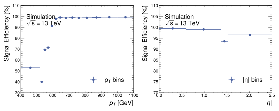
This section presents the results from the tests performed on the best-performing DNN jet tagger. The hyperparameters for this classifier model are contained within Table 5. The signal and the backgrounds classification performance was broadly the same across all top five models. Therefore, the main criteria for differentiation of these models was the effectiveness of the transverse momentum and pseudorapidity bin weighting. The best model of these top five models was the model with the smallest variation in signal efficiency for both the transverse momentum and pseudorapidity bins. The best model’s signal efficiency curves with respect to these features can be seen in Figure Fig. 5. The best model was trained again with rounded hyperparameter values; all figures contained in this section are from this final training procedure.
| Hyperparameter | Value |
|---|---|
| Training epochs | 30 |
| Early stopping | 27 |
| Optimiser | Adam |
| Dropout probability | 0.03 |
| Learning rate | 0.001 |
| Hidden layers | 4 |
| Hidden nodes | 200 |
| Activation function | ReLU |
The training curves for the DNN are displayed in Figure Fig. 6. The left-hand side plot shows the cross-entropy loss as a function of the training epochs on both the training and validation datasets, whereas the right-hand side plot shows the signal accuracy as a function of the training epochs. The training curves are typical for DNN training, with training performance better than validation performance. The loss curves exhibit the classic shape with little fluctuation. When examining the gap between training and validation loss curves, it should be noted that the difference between the training loss at the first and last epochs is small at \(0.025\). On the other hand, whilst signal performance shows a trend of increased performance, it fluctuates more significantly. It should be noted that the signal accuracy is always greater than \(98.8\%\); however, this fluctuation motivated the use of the cross-entropy loss as the hyperparameter optimisation criterion.

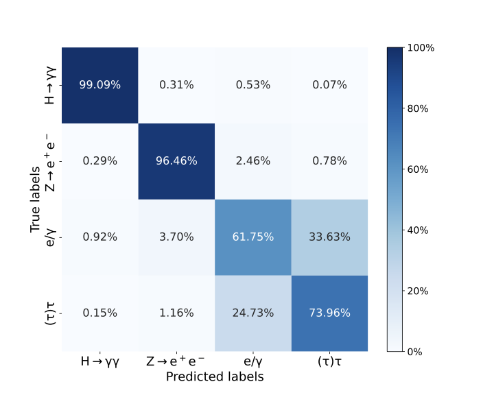
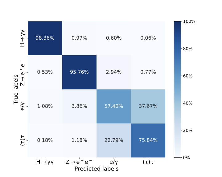
Of the evaluation methods, per jet classification performance is examined first, using the confusion matrix in Figure Fig. 7. Each jet in the input data is assigned to its highest softmax probability value produced by the DNN. This is then compared to the true jet classification to produce a percentage value. There is a high degree of signal separation with \(99.09\%\) of the signal jets correctly identified. There is little confusion between the signal and background classes; the most confusion occurs with the \(e/\gamma\)-jets with the DNN incorrectly predicting these jets \(0.53\%\) of the time when the true class is the signal. False positives are slightly more common, with the signal class being predicted \(0.29\%\), \(0.92\%\) and \(0.15\%\) for each background \(Z\rightarrow e^+e^-\), \(e/\gamma\) and \((\tau)\tau\) respectively.
The confusion between the background jets is significantly greater, especially between \(e/\gamma\) and \((\tau)\tau\)-jets. The highest degree of confusion between the DNN outputs occurs when the DNN incorrectly predicts a jet is a \((\tau)\tau\)-jet when it is, in fact, a \(e/\gamma\)-jet. This particular instance of confusion occurs at a rate of \(33.63\%\).
Table 6 contains the DNN AUC values. The performance of the DNN over all classes is extremely high, with the \(H\rightarrow\gamma\gamma\) and \(Z\rightarrow e^+e^-\)-jets possessing the maximum or near-maximum AUC score. No AUC score is lower than \(0.91\), indicating high capability by the DNN classifier.
| Jet | DNN AUC Score | ANN AUC Score |
|---|---|---|
| \(H\rightarrow\gamma\gamma\) | 1.00 | 1.00 |
| \(Z\rightarrow e^+ e^-\) | 0.99 | 0.99 |
| \(e/\gamma\) | 0.93 | 0.92 |
| \((\tau)\tau\) | 0.91 | 0.90 |
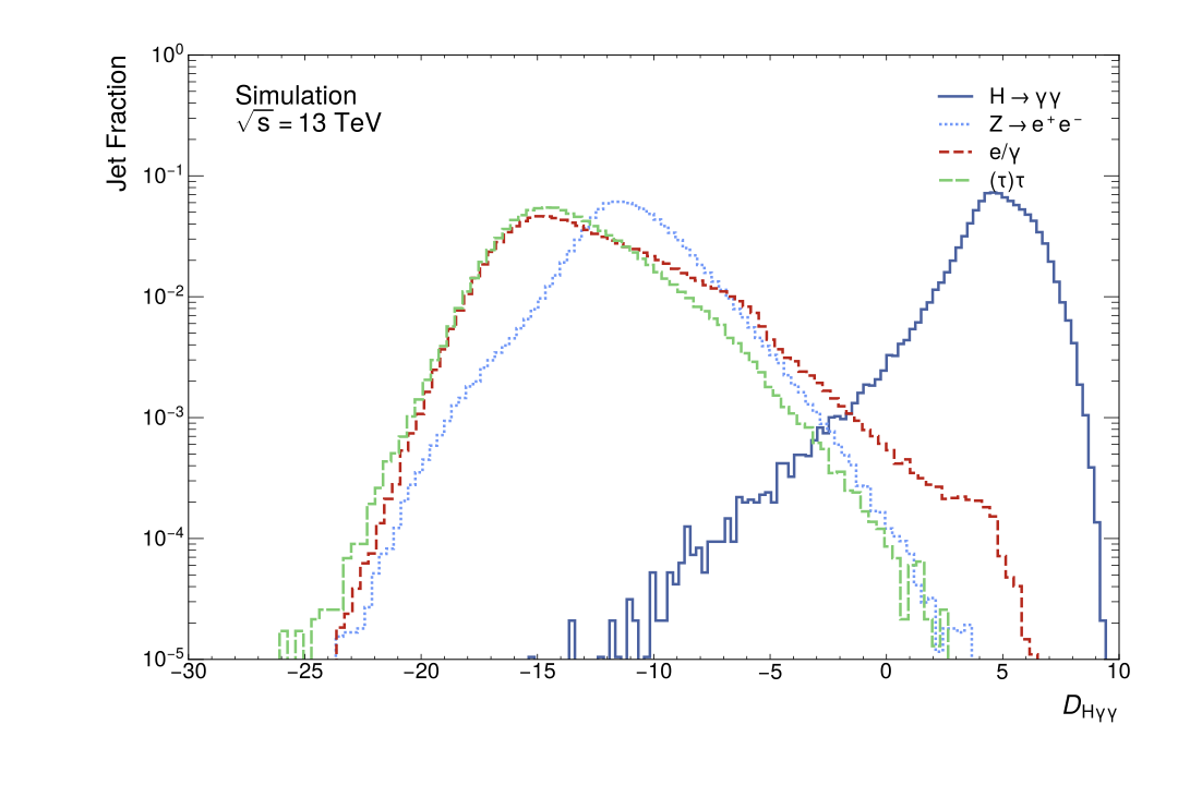
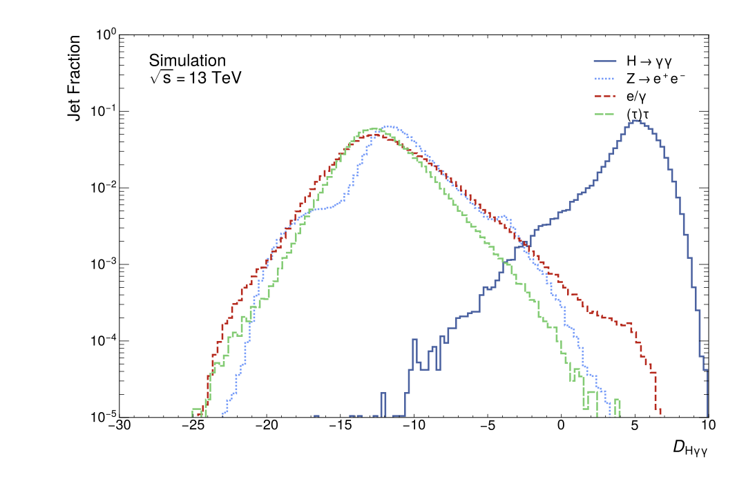
In Figure Fig. 8, the distribution of the scalar discriminant \(D_{H\gamma\gamma}\) score is presented. This distribution is with respect to the fraction of the jets in the data sample for each jet class. A high degree of separation between the signal and the background jets can be observed. The distributions of the backgrounds are relatively similar to one another with peaks of \(D_{H\gamma\gamma}\in(-17,-10)\) whereas the signal \(D_{H\gamma\gamma}\) peak is around \(5\). Additionally, it should be noted that the \(D_{H\gamma\gamma}\) score is most similar between the \(e/\gamma\) and \((\tau)\tau\)-jets with the peaks around \(-17\). The \(D_{H\gamma\gamma}\) is around \(-12\) for the \(Z\rightarrow e^+e^-\) decays. This is similar to the other experimental results that indicate the ability of the DNN to discriminate between the backgrounds is weakest between \(e/\gamma\) and \((\tau)\tau\)-jets.
The scalar discriminant is also used with mutual information to interpret the importance of different feature variables to the DNN output discriminant. This information is contained in Table 3.5 and provides the features and their mutual information scores with \(D_{H\gamma\gamma}\). Importantly, the mass feature has the greatest mutual information score and is thus the most important feature of the DNN jet tagger.
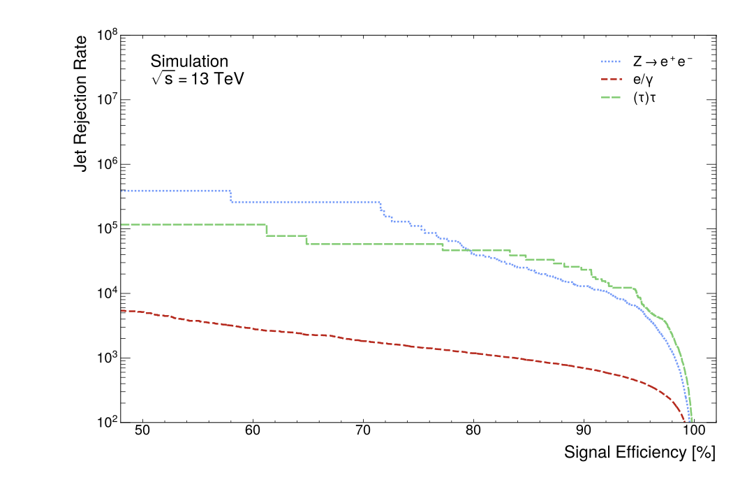
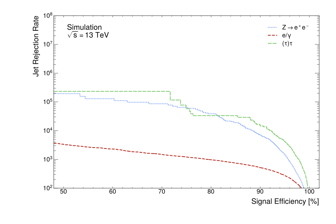
Figure Fig. 9 displays the jet rejection rate per background jet as a function of the signal efficiency. As is typical for these curves, performance is degraded at higher signal efficiencies as more background jets are accepted as signal jets. The less smooth curves produced for the \(Z\rightarrow e^+e^-\) decays and \((\tau)\tau\)-jets indicate a lack of MC statistics for these background jets at lower signal efficiencies.
3.2 ANN
This section presents the results from the ANN jet tagger. The same evaluation figures and tables are used as in the previous section to allow direct comparison to the DNN jet tagger. Additionally, jet rejection rates for the background jets as a function of the mass bins are included. These are created for both DNN and ANN jet taggers to display the effect of adversarial training on mass correlation.
Table 7 contains the hyperparameters found during the grid search optimisation. A final ANN classifier was trained using rounded values from the hyperparameter optimisation. Notably, the two learning rates are orders of magnitude different from the learning rate found for the DNN. Additionally, the adversary was found to be a less complex and expressive network than the classifier.
Figure 3.6 contains the confusion matrix of the ANN classifier subnetwork. Performance is broadly similar to the DNN, with slightly more confusion occurring, but this is a relatively minimal degradation in performance.
Figures 3.7 and 3.8 are the scalar discriminant distributions and jet rejection rates, respectively. Both of these figures are highly similar to those produced for the DNN; however, there is a greater difference in rejection rate at lower signal efficiencies for the ANN jet taggers, but these are small distinctions between the tagging networks. Table 6 shows that the DNN possesses mildly better AUC scores for \(e/\gamma\) and \((\tau)\tau\)-jets than the DNN, although the DNN and ANN have the same AUC scores for the signal and \(Z\rightarrow e^+e^-\)-jets.
| Hyperparameter | Value |
|---|---|
| \(\lambda\) | 0.01 |
| Training epochs | 30 |
| Early stopping | 16 |
| Optimiser | Adam |
| Dropout probability (C) | 0.01 |
| Learning rate (C) | 0.01 |
| Hidden layers (C) | 4 |
| Hidden nodes (C) | 200 |
| Activation function (C) | ReLU |
| Learning rate (A) | 1 |
| Hidden layers (A) | 4 |
| Hidden nodes (A) | 100 |
| Activation function (A) | ReLU |
In Table 3.5, the mutual information score between the features and the scalar discriminant is presented. In absolute value, the greatest change between this metric for the DNN and ANN is the -0.10 change in the mutual information between the mass and \(D_{H\gamma\gamma}\). This corresponds to a percentage change of \(-27.8\%\), the second-greatest percentage change decrease after the \(\max{(E_{layer}/E_{jet})}\) feature. Several features undergo much larger percentage change increases; the greatest is the mutual information score for the \(|\eta|\) bin with \(D_{H\gamma\gamma}\), which undergoes a \(175.0\%\) increase.
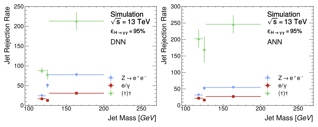
Figure Fig. 10 contains two subplots displaying the background jet rejection rates as a function of mass at the \(\epsilon_{H\rightarrow\gamma\gamma}=95\%\) operating point for both the DNN and ANN jet taggers. Only three mass bins satisfy this criterion: those closest to the signal mass. It can be seen in this figure that the distributions of both \(Z\rightarrow e^+e^-\) and \(e/\gamma\)-jets are slightly flatter, and the jet rejection rate for the \((\tau)\tau\)-jets are greater for the ANN. Total jet rejection rates derived from figures Fig. 9 and 3.8 at the same operating point are contained in Table 8. The DNN outperforms the ANN in reducing background jets at this operating point in this more general metric.
| Rejection Rates at \(\epsilon_{H\rightarrow\gamma\gamma}=95\%\) | ||
|---|---|---|
| 2-3 Background Jet | DNN | ANN |
| \(Z\rightarrow e^+e^-\) | 7401 | 1469 |
| \(e/\gamma\) | 448 | 275 |
| \((\tau)\tau\) | 8955 | 4312 |
| Feature | DNN MI | ANN MI | \(\Delta\)MI | \(\Delta\)MI [%] |
|---|---|---|---|---|
| \(m\) | 0.36 | 0.26 | -0.10 | -27.8 |
| \(r^{(\beta=1)}_{N=1}\) | 0.21 | 0.21 | 0.00 | 0.0 |
| \(E/p\) | 0.17 | 0.21 | +0.04 | +23.5 |
| \(N^{Trks}\) | 0.25 | 0.20 | -0.05 | -20.0 |
| \(f_{EM}\) | 0.18 | 0.15 | -0.03 | +16.7 |
| \(\max{(\frac{E_{layer}}{E_{jet}})}\) | 0.21 | 0.14 | -0.07 | -33.3 |
| \(p_T\) Bin | 0.12 | 0.12 | 0.00 | 0.0 |
| \(\Delta R(c_1,c_2)\) | 0.14 | 0.12 | -0.02 | -14.3 |
| \(N^{Const.}\) | 0.14 | 0.11 | -0.03 | 21.4 |
| \(|\eta|\) Bin | 0.04 | 0.11 | +0.07 | +175.0 |
| \(\Delta R(c_2,j)\) | 0.11 | 0.10 | -0.01 | -9.1 |
| Planar Flow | 0.12 | 0.09 | -0.03 | -25.0 |
| Balance | 0.03 | 0.06 | +0.03 | +100.0 |
| Width | 0.06 | 0.04 | -0.02 | -33.3 |
| \(\Delta R(c_1,j)\) | 0.04 | 0.03 | -0.01 | -25.0 |
4 Discussion
4.1 DNN
The overall performance of the DNN jet tagger is strong. It has a high signal classification rate at \(99.09\%\) and a high value for the other heavy boson \(Z\rightarrow e^+e^-\) identifications at \(96.46\%\) seen in the confusion matrix in Figure Fig. 7. The DNN correctly predicts the \(Z\rightarrow e^+ e^-\) decays to a high degree, supporting this architecture’s use for highly boosted, heavy boson identification. High AUC scores seen in Table 6 for the signal (1.00) and \(Z\rightarrow e^+ e^-\) decays (0.99) support this. It should be noted that the AUC scores are high for the other backgrounds, both above 0.90; for signal and \(Z\rightarrow e^+ e^-\) decays, they are near the possible maximum. The distribution of the scalar discriminant \(D_{H\gamma\gamma}\) as seen in Figure Fig. 8 is very similar to the distribution of the related scalar discriminant \(D_{Zee}\) for \(Z\rightarrow e^+ e^-\) decays seen in previous work (ATLAS Collaboration 2022a). This indicates that the DNN jet tagger performs similarly to the jet tagging scenario in which it was previously implemented.
The DNN jet tagger achieves high background jet rejection rates for all backgrounds, as seen in Figure Fig. 9. The MC statistics are insufficient for the \(Z\rightarrow e^+ e^-\) decays and \((\tau)\tau\)-jets, as evidenced by the curves possessing large steps at lower signal efficiencies. This motivates using a high signal efficiency as an operating point for the jet tagger as it remains on a smooth part of the curve. This reason, combined with its previous use as the highest (tight) operating point in related work (ATLAS Collaboration 2022a) and the need for high efficiency for boosted Standard Model searches, motivates the choice of \(\epsilon_{H\rightarrow\gamma\gamma}=95\%\). Future work may also generate more MC statistics so as to use lower operating points to assess the DNN, as related work uses multiple operating points (ATLAS Collaboration 2022a). The highly boosted \(H\rightarrow\gamma\gamma\) decays DNN jet tagger developed in this work at the same operating point performs 39.5% worse on reducing \(e/\gamma\)-jets than the related highly boosted \(Z\rightarrow e^+ e^-\) jet tagger (ATLAS Collaboration 2022a). The rejection rate in Table 8 for \(e/\gamma\)-jets is in the same order as the previous result (ATLAS Collaboration 2022a). However, the DNN jet tagger developed here has an increased rejection rate for \((\tau)\tau\)-jets of 1029.3% compared to the previous study (ATLAS Collaboration 2022a). Such a stark increase may reflect the difference in the distribution of MC-generated jets in the training dataset. Nonetheless, the DNN jet tagger is significantly more successful at reducing the \((\tau)\tau\)-jets than the previous study. The DNN jet tagger is also highly successful at reducing the \(Z\rightarrow e^+ e^-\) decays; the rejection rate at the \(\epsilon_{H\rightarrow\gamma\gamma}=95\%\) is of the same order as the rejection rates for the \((\tau)\tau\)-jets which have been noted as high.
The best-performing DNN was selected based on the flatness of the signal efficiency curves with respect to the transverse momentum and pseudorapidity bins. These data are shown in Figure Fig. 5; performance strongly degrades at low transverse momentum bin values and the highest pseudorapidity bin value. The signal efficiency distribution largely follows the data distribution seen in Figure Fig. 2. This indicates that weighting the loss function to have a flat distribution with respect to the classes has a limited effect as it does not overcome the inherent data distribution. This is a limitation of the DNN jet tagger as the method of weighting the loss function to be flat with respect to these features is proving limited in its success.
The DNN jet tagger’s performance aligns with related work for a highly boosted \(Z\rightarrow e^+e^-\) decays (ATLAS Collaboration 2022a), showing this architecture effectively identifies different jets using the ATLAS detector. The effectiveness of weighting the loss function to have a flat distribution with respect to the \(p_T\) and \(|\eta|\) bins has, however, been identified as questionable due to its mirroring of the data distribution when the signal efficiency is calculated for these feature bins. A more complex method may be required in future work to improve identification invariance with respect to the transverse momentum and pseudorapidity bins.
4.2 ANN
The performance of the jet tagging sub-network of the ANN setup is a modicum worse than the DNN. Comparing the confusion matrices between these two classifiers, the ANN jet tagger is \(-0.73\%\) less accurate on the signal classification. The ANN is \(-0.70\%\) worse performing on \(Z\rightarrow e^+ e^-\) decay classification and \(-4.35\%\) for the \(e/\gamma\) class. It performs slightly better on \((\tau)\tau\)-jets with a \(+1.88\%\) increase. All class confusion is approximately similar between the DNN and ANN. The \(D_{H\gamma\gamma}\) distributions share the same attributes, and a clear separation between the background and signal jets is easily observed. The jet rejection rates of the background jets at the \(\epsilon_{H\rightarrow\gamma\gamma}=95\%\) are about half for the \(e/\gamma\) and \((\tau)\tau\)-jets when compared to the DNN, as seen in Table 8. The most significant degradation in rejection rate is for the \(Z\rightarrow e^+ e^-\) decays, which is \(-80.2\%\) for the ANN compared to the rejection rate of the DNN jet tagger. Therefore, attempting to reduce the bias and sensitivity to the mass feature has reduced the ability of the jet tagger to reduce the background jets. However, in Figure Fig. 10, the effect on jet rejection rate as a function of mass between the DNN and ANN can be seen. In this metric, the distribution of rejection rates for all the background jets is somewhat flattened, and there is a clear increase in the rejection rate of the \((\tau)\tau\)-jets. Unfortunately, only the three mass bins closest to the signal mass satisfy the operating point criterion. The case for both the DNN and ANN is due to the availability of signal MC statistics in the data and could be mitigated by a differently generated dataset.
The ability of the jet tagger to classify the signal and reduce backgrounds is comparable to the ability of the DNN. How it uses the available information in the features is of significant interest as reducing dependence on one feature may reasonably suggest that other features are utilised more. Table 3.5 contains the mutual information between the feature variables and the scalar discriminant of the jet taggers. As reported in Table 3.5, the greatest absolute change in mutual information score occurs with the mass feature. This strongly indicates that this feature’s adversarial training targeting decorrelation has occurred as intended. It should be noted that the mass feature still possesses the highest mutual information with the discriminant. Four features increased their mutual information score with the discriminant, \(E/p\), \(f_{EM}\), \(|\eta|\) bin and the balance. These features are not strongly associated with the mass, so it is reasonable that the network would learn more from these features than the DNN did to compensate for the reduced importance of the mass feature. The increased dependence on the \(|\eta|\) bin feature is relatively large in absolute and percentage terms. This is an issue as it is attempted to make the network decorrelated to this feature by weighting the loss function during the training. Whilst this is a concern and may warrant more attention to the invariance of this feature in the future, the \(|\eta|\) bin dependence is now in line with the transverse momentum bin feature for which the mutual information score has remained unchanged between the DNN and ANN. Dependence on \(f_{EM}\) has increased; this result is understandable due to the di-photon decay products of the signal jet, which has a relatively distinct distribution from the \(e/\gamma\) and \((\tau)\tau\)-jets, as seen in Figure Fig. 3. However, its similarity to the \(Z\rightarrow e^+ e^-\) decays may explain why the ANN jet tagger has not utilised this feature even more. Interestingly, there is no change in the mutual information score between the jet substructure feature \(r^{(\beta=1)}_{N=1}\) and the discriminant, comparing the DNN and the ANN. It does, however, become the second most important feature due to the decrease in the importance of the multiplicity of the tracks per jet. So, relatively, the substructure feature of the jet becomes more influential in the decision process of the jet tagger.
As mentioned, the ability of the ANN jet tagger to learn to decorrelate from the mass is highly influenced by the availability of examples of the jets in each mass decile bin. This has limited the ability of the ANN to decorrelate from mass evenly in different regions of the mass due to the availability of MC statistics from signal events. As MC-generated signal jets are clustered around the Higgs boson mass at 125.09 GeV (ATLAS and CMS Collaborations 2015), examples at lower masses, particularly, are limited. The same datasets for training, validation and testing were used for the ANN and the DNN. In future efforts employing the ANN architecture for feature decorrelation, a significant focus should be on generating MC events that are more suitable for this task. Allowing a broader distribution of signal masses around the peak of 125.09 GeV should immediately improve the distribution of the examples in the data and improve the ability of the ANN to learn to identify jets and decorrelate from the mass more easily across a greater mass range.
It should also be noted that related work in mass-decorrelated jet tagging has been done in binary classification scenarios, a signal class and a combined backgrounds class (C. Shimmin et al. 2017; Cheng and Courville 2022; Cheng et al. 2023). Thus, this multiclass classification task that has been set is inherently more complex than previous work. This may explain why the degree of mass invariance seen in related work is greater than what has been determined in this thesis.
In summary, the ANN jet tagger’s performance is qualitatively and quantitatively similar to the DNN network, which has been shown effective to the same order as previous work on another highly boosted heavy boson (ATLAS Collaboration 2022a). This suggests that the ANN jet tagger is at least a viable architecture in classification ability compared to another functioning jet tagger architecture. There has been a 27.8% reduction in the dependence on the mass variable as measured using the mutual information between the feature and the discriminant \(D_{H\gamma\gamma}\). Combined with the flattened distributions of the background jet rejection rates for the three operating point satisfying mass bins, there is good evidence that this approach has somewhat decorrelated the jet tagger’s identifications from the mass feature data. This decorrelation is limited, with the most likely culprit for the limitation identified as the distribution of the MC-generated training data with respect to mass. As the datasets used are MC generated, engineering this data to tailor the training scenario to the ANN setup is likely the single most effective recommendation to improve the mass invariance of the identifications made by the ANN jet tagger.
4.3 Directions for Future Research
The previous sections of this chapter discussed the capabilities and limitations of the developed jet taggers. The found limitations motivate directions for future research as mitigating or entirely avoiding these limitations come from three main areas. The first route is better hyperparameter optimisation, thus searching for a better model within the described architecture. The second is to extend the ANN feature decorrelation technique to other features for which reduced sensitivity and bias are desirable.
4.3.1 Hyperparameter Optimisation
The hyperparameter grid search spaces were defined based on the results found in previous and related work (ATLAS Collaboration 2022a; C. Shimmin et al. 2017). However, a different hyperparameter optimisation technique may be more appropriate for both networks, especially the ANN jet tagger, due to its significantly greater number of hyperparameters.
One such method is random search; a hyperparameter space is defined, and the hyperparameter combinations are then randomly selected from this space (Bergstra and Bengio 2012). This comes with significant benefits, especially when dealing with many hyperparameters. First, computational efficiency: random search usually requires fewer trials to find a good set of hyperparameters compared to grid search (Bergstra and Bengio 2012). Secondly, random search can explore a larger hyperparameter space in a given amount of time than grid search (Bergstra and Bengio 2012). Random search also does not waste resources computing very similar hyperparameter combinations. Finally, random search can converge to an optimal solution faster than grid search for larger hyperparameter spaces (Bergstra and Bengio 2012). In this thesis, the hyperparameter space was restricted to make the research compatible with the computational and time resources available; even with this limitation, a proof-of-concept ANN model was found. A greater hyperparameter space can be searched using random search to improve hyperparameter optimisation efficiency, and a better-performing ANN \(H\rightarrow\gamma\gamma\) decays jet tagger will likely be found.
4.3.2 Extending ANN to Other Features
The jet tagger developed using adversarial training has measurably reduced systematic uncertainties by reducing the bias on the mass feature variable compared to the DNN jet tagger. This was done using a regularising term in the loss function for the mass feature that was determined by the powerful and flexible adversary DNN. However, there are concerns about the jet tagger being relatively sensitive to the transverse momentum and pseudorapidity of the decay products. This was handled by weighting the loss function with respect to these features. This method is less effective than desired, as seen for the DNN. Applying the adversarial network architecture and training to the transverse momentum and pseudorapidity may be quite effective, especially as these features are much less strongly correlated to other features than the mass feature. This can be seen in the correlation plot in Figure Fig. 4.
One could create one ANN setup per feature from which the jet tagger output is to be decorrelated, then create an ensemble of these networks (Breiman 1996). The ensemble approach would simplify training significantly as a single jet tagger per decorrelated feature variable would be required instead of regularising all \(N\) features in a single complex training setup. Each training scenario would then be on par with what has been developed and shown to have the desired effect in this thesis. At inference time, the \(N\) jet taggers would vote on the jet class (Breiman 1996). The weighting of the jet taggers in the ensemble can then be tuned to a user’s specific requirements. Ensembles are generally better than single classifiers as they tend to be more accurate than their constituent parts (Dietterich 2000). This is because they can capture different representations in the data and pool this information into the final output classification (Dietterich 2000). Training could also be highly parallelised as each ANN could be trained independently, reducing the computational expense of training a single highly complex adversarial training scenario.
Developing further ensemble ANN jet taggers would allow the taggers to be more general and would likely be effective for more boosted decays that result in two photons. This would allow the legitimate use of such a general jet tagger for searches of hypothetical particles such as additional Higgs bosons (R. Barbieri et al. 2013), axion-like particles (M. Bauer et al. 2017), and various dark matter candidate particles (Kahlhoefer 2017).
In the next and final chapter, conclusive remarks highlight this thesis’s key contributions and outcomes.
5 Conclusions
In this thesis, two jet tagging algorithms have been developed and presented to identify highly boosted \(H\rightarrow\gamma\gamma\) decays using the ATLAS detector at the LHC. The first jet tagging algorithm based on the DNN architecture was found to perform to a similar level as a related jet tagger used for highly boosted \(Z\rightarrow e^+ e^-\) decays. Noise from the background jets was reduced to a similar degree. Additionally, some performance improvements were observed in the \(H\rightarrow\gamma\gamma\) jet tagger, which was found to reject \((\tau)\tau\)-jets at a higher rate than the related jet tagger. Thus, the research aim of creating a robust jet tagging algorithm for highly boosted \(H\rightarrow\gamma\gamma\) decays has been achieved.
The second jet tagger developed using adversarial training was found to have a slightly degraded performance compared to the DNN jet tagger. However, this performance reduction was overall relatively mild, meaning the ANN jet tagger could still be reliably used to detect \(H\rightarrow\gamma\gamma\) decays. A \(27.8\%\) reduction in mutual information between the mass and scalar discriminant was found between the DNN and ANN jet taggers. Indicating a reduction in the importance of the mass feature to the jet tagger’s decision-making. There is also evidence that the rejection rates for the background jets have a flatter distribution compared to the DNN at the \(95\%\) operating point.
The evidence for improved mass-decorrelated classification predominantly indicates what can be achieved; several recommendations have been made to move beyond this proof-of-concept mass-decorrelated jet tagger to an actual tool for LHC experiments. The most important of these to improve the ANN jet tagger is to MC-generate the jet statistics purposefully with downstream ANN training in mind. This would involve generating \(H\rightarrow\gamma\gamma\) decays with a significantly broader mass peak. Additional recommendations for the ANN are to change the hyperparameter optimisation method to random search to increase the explored hyperparameter space and to create ensembles of these jet taggers. These are the methods for further developing a mass-decorrelate ANN jet tagger and reducing the limitations found in this thesis.
Thus, the second research aim to produce a mass-decorrelated jet tagger is shown to be possible. Still, considerable work and further research must be done to make this model sufficiently insensitive to mass to reduce the systematic bias caused by the mass to a significant degree. This is especially the case due to the much higher complexity of the ANN than the DNN jet tagger, which is much cheaper to develop.
To conclude, the research aims have either been fully achieved or robust progress has been made to achieve them. Jet tagging algorithms of sufficient sensitivity have been developed to improve the detection of highly boosted Higgs boson di-photon decays in the ATLAS detector. Thus furthering the search for new physics in discovering properties beyond the Standard Model and the search for discrepancies within the Standard Model.
References
Where \(c\) is the speed of light in natural units, therefore \(c=1\).↩︎
ATLAS has a right-handed coordinate system that originates at the interaction point (IP) in the detector’s centre (ATLAS Collaboration 2022a). From the IP, the \(z\)-axis follows the beam pipe; the \(x\) and \(y\)-axes point to the LHC ring centre and upwards, respectively (ATLAS Collaboration 2022a). Cylindrical coordinates \((r, \phi)\) measure in the transverse plane with \(\phi\) as the azimuthal angle about the \(z\)-axis (ATLAS Collaboration 2022a). Pseudorapidity \((\eta)\) is in terms of the polar angle \((\theta)\), \(\eta = -\ln \tan(\theta/2)\), and angular distance is \(\Delta R \equiv \sqrt{(\Delta\eta)^{2} + (\Delta\phi)^{2}}\) (ATLAS Collaboration 2022a).↩︎
The angular distance \(\Delta R\) of a two-body decay can be approximated by \(\Delta R \approx \frac{2m}{p_T}\) where \(m\) is the parent particle mass and \(p_T\) is its transverse momentum.↩︎